How to Remove Duplicates in Excel (6 Method That Actually Works)

Duplicate data is one of the most common Excel problems. It messes up your counts, inflates your totals, and makes your reports unreliable. The good news is Excel gives you multiple ways to remove duplicates, and most of them take under a minute.

The Fastest Way to Remove Duplicates in Excel

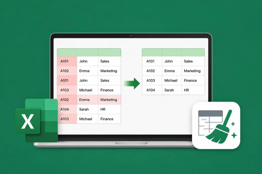
If you just want duplicates gone right now, here it is:

1. Click anywhere inside your data
2. Go to the Data tab
3. Click Remove Duplicates
4. Choose which columns to check
5. Click OK

Excel tells you how many duplicates were removed and how many unique values remain. That’s it. For most people, this is all they need.

But keep reading if your situation is more complicated, because the built-in Remove Duplicates tool has real limitations.

What “Duplicate” Means in Excel

Before you start deleting rows, be clear on what counts as a duplicate in your dataset.

Excel considers a row a duplicate when every selected column matches exactly. So if you select only the “Name” column, two rows with the same name but different email addresses both get flagged, even if they’re actually different people.

A few things to know:

• Excel comparisons are not case-sensitive by default. “JOHN” and “john” are treated as the same value.
• Trailing spaces can fool Excel. “Apple ” and “Apple” may or may not be considered duplicates depending on your method.
• Blank cells are treated as values. Two blank cells in the same column count as duplicates.

Always decide which columns define a “true” duplicate before you touch anything.

Method 1: Remove Duplicates Tool (Built-in)

This is the quickest method and works for most straightforward cases.

Steps

1. Select your data range or click any cell inside your table
2. Go to Data > Remove Duplicates
3. A dialog box appears showing all your columns
4. Check the columns that should all match for a row to be considered a duplicate
5. Click OK

Excel removes duplicate rows and keeps the first occurrence of each unique combination. The deleted rows are gone permanently unless you undo immediately with Ctrl+Z.

When to Use It

• You have a clean, flat table
• You want a permanent deletion
• You don’t need to see which rows were removed

Limitation

It deletes data right away. There’s no preview. If you want to review duplicates first, use a different method.

Method 2: Highlight Duplicates First (Then Decide)

If you want to see duplicates before removing them, use Conditional Formatting to flag them visually.

Steps

1. Select the column or range you want to check
2. Go to Home > Conditional Formatting > Highlight Cell Rules > Duplicate Values
3. Choose a highlight color and click OK
4. Review the highlighted cells
5. Manually delete rows you want to remove, or filter by color and delete

This approach gives you control. You see exactly what’s getting flagged before anything is deleted.

Tip

You can sort by color after highlighting. Go to Data > Sort, then sort by cell color so all duplicates rise to the top. Easier to review that way.

Method 3: Use COUNTIF to Find Duplicates Without Deleting

Sometimes you don’t want to delete anything yet. You just want to identify which rows are duplicates. COUNTIF handles this well.

Formula

In a blank column next to your data, type:

=COUNTIF($A$2:$A$100, A2)

This counts how many times the value in A2 appears in the range. Any number greater than 1 is a duplicate.

To label them more clearly:

=IF(COUNTIF($A$2:A2, A2)>1, "Duplicate", "Unique")

This version labels the second and subsequent occurrences as duplicates while keeping the first. Drag it down the column and you get a clear picture of your data.

Once labeled, you can filter on “Duplicate” and delete those rows.

Method 4: Advanced Filter for Unique Records

Advanced Filter is an underused tool that copies unique records to a new location without touching your original data.

Steps

1. Select your data range including headers
2. Go to Data > Advanced
3. Choose Copy to another location
4. In “Copy to,” select a blank cell where you want the clean data to appear
5. Check Unique records only
6. Click OK

Your original data stays untouched. The filtered unique records appear in the new location. This is great when you need a clean copy but want to keep the original for reference.

Method 5: UNIQUE Function (Excel 365 and Excel 2021)

If you’re on Microsoft 365 or Excel 2021, the UNIQUE function is the cleanest solution. It returns a list of unique values dynamically.

Formula

=UNIQUE(A2:A100)

For multiple columns:

=UNIQUE(A2:C100)

The result spills into adjacent cells automatically. If your source data changes, the unique list updates too. No manual steps needed.

Extended Use

Want only values that appear exactly once (not even duplicated once)?

=UNIQUE(A2:A100, FALSE, TRUE)

The third argument set to TRUE returns values that appear only one time in the dataset.

This function is a game changer for dynamic reports. Microsoft’s support documentation covers UNIQUE in detail if you want to dig deeper into its arguments.

Method 6: Power Query for Large or Recurring Datasets

For large datasets or situations where you remove duplicates regularly, Power Query is the right tool. It’s repeatable, non-destructive, and handles thousands of rows easily.

Steps

1. Click inside your data
2. Go to Data > From Table/Range (this loads the data into Power Query)
3. Select the columns that define a duplicate
4. Go to Home > Remove Rows > Remove Duplicates
5. Click Close & Load

Power Query loads the cleaned data into a new sheet. Your original data is untouched. Next time you need to repeat the process, just refresh the query.

This method is especially useful for monthly or weekly data cleaning tasks. You set it up once, and from then on it’s a one-click refresh.

Comparing All Methods at a Glance

Method	Deletes Original Data	Preview Before Deleting	Works in Older Excel	Dynamic/Refreshable
Remove Duplicates Tool	Yes	No	Yes	No
Conditional Formatting	No	Yes	Yes	No
COUNTIF Formula	No	Yes	Yes	No
Advanced Filter	No	No	Yes	No
UNIQUE Function	No	Yes	365/2021 only	Yes
Power Query	No	Yes	2016+	Yes

How to Remove Duplicates Based on One Column Only

A very common scenario: you have a dataset with multiple columns but you only want to find duplicates based on one specific column, like email address or product ID.

With the Remove Duplicates tool, just uncheck all columns in the dialog and check only the one that matters. Excel will remove rows where that column repeats, keeping the first occurrence.

With COUNTIF, lock the column reference:

=COUNTIF($B$2:$B$100, B2)>1

Only column B is checked. The rest of the row doesn’t matter.

How to Remove Duplicates but Keep the Last Occurrence

By default, Excel keeps the first duplicate and removes the rest. What if you want to keep the most recent entry?

Reverse your data first. Sort it in reverse order (newest first), run Remove Duplicates, then sort it back. Now the “first occurrence” Excel keeps is actually the most recent one.

Or use this COUNTIF trick. In a helper column:

=COUNTIF(A2:$A$100, A2)

Note the mixed reference. This counts how many times the value appears from the current row to the end of the list. A result of 1 means it’s the last occurrence. Filter for 1 and keep those rows.

Handling Duplicates Across Multiple Sheets

Excel’s Remove Duplicates tool doesn’t work across sheets. If you need to find duplicates between Sheet1 and Sheet2, you need a formula approach.

On Sheet2, add a helper column:

=COUNTIF(Sheet1!$A$2:$A$100, A2)

Any result greater than 0 means that value already exists on Sheet1. Filter and delete as needed.

For complex cross-sheet work, Power Query can combine multiple sheets first, then deduplicate the combined result. The Excel Jet resource has solid examples of formula-based duplicate detection worth bookmarking.

Common Mistakes to Avoid

Not backing up first. Remove Duplicates is permanent. Always save a copy before you run it or work on a duplicate of the file.

Selecting the wrong columns. If you include a unique ID column in your Remove Duplicates check, nothing will be removed because every row has a different ID.

Ignoring leading/trailing spaces. “Apple” and “Apple ” look identical but aren’t. Use TRIM to clean your data first if spaces might be an issue:

=TRIM(A2)

Assuming case matters. Excel’s built-in duplicate tools are case-insensitive. If case matters in your data, you need a custom formula approach using EXACT().

Working on raw data without a backup. Always. Make. A. Backup.

Before You Remove Duplicates: A Quick Checklist

• Saved a backup copy of the file
• Decided which columns define a true duplicate
• Checked for leading/trailing spaces that might cause false positives
• Decided whether to keep the first or last occurrence
• Decided if you want to preview duplicates first or delete immediately

Conclusion

Removing duplicates in Excel doesn’t have to be complicated. For a quick cleanup, the Remove Duplicates tool under the Data tab gets the job done in seconds. For more control, COUNTIF lets you label duplicates before deleting anything. For recurring work, Power Query is worth learning once and using forever. And if you’re on Excel 365, UNIQUE is simply the cleanest way to extract a deduplicated list.

FAQs

Does Excel’s Remove Duplicates tool work on filtered data?

It does not respect active filters. Even if you have a filter applied showing only certain rows, Remove Duplicates runs on the entire dataset, including hidden rows. If you only want to remove duplicates from visible rows, copy the filtered results to a new sheet first, then run Remove Duplicates there.

Can I undo Remove Duplicates after closing and saving the file?

No. Once you save and close, the undo history is gone. The deleted rows cannot be recovered unless you have a backup. This is why saving a copy before running the tool matters so much.

Why does Excel say “0 duplicates found” when I can clearly see repeated values?

This usually happens because the repeated values are not actually identical. Common causes are extra spaces, different formatting (text vs. number), or invisible characters. Use TRIM and CLEAN on your data, and make sure the column format is consistent, before running the check again.

Is there a way to remove duplicates in Excel without a helper column or formula?

Yes. You can use Advanced Filter with “Unique records only” checked. It extracts unique rows to a new location without any formulas. Power Query’s Remove Duplicates step also does this cleanly, no helper columns needed.

Does the UNIQUE function update automatically when new data is added?

It updates when the source range includes new data, but only if the range reference covers those new rows. If your formula references A2:A100 and new data goes in A101, it won’t be included. Use a named Table as your source instead. When you reference a Table column, UNIQUE automatically picks up new rows added to the Table.