
Comparing two columns in Excel sounds simple until you’re staring at 5,000 rows trying to figure out what’s different. I’ve been there. The good news is Excel gives you several ways to do this, and once you know them, you’ll handle it in minutes instead of hours.
The Fastest Way to Compare Two Columns in Excel
If you just need a quick visual scan, select both columns, go to Home > Conditional Formatting > Highlight Cell Rules > Duplicate Values, and Excel will color-code matches or differences instantly. Takes about 10 seconds.
But if you need something more precise, keep reading.
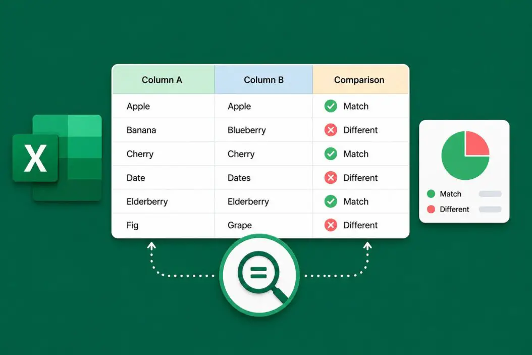
Using IF Formula to Compare Two Columns Row by Row
This is the most common approach. It checks each row and tells you whether the values match.
Say your data is in column A and column B, starting at row 2. In column C, type:
=IF(A2=B2,"Match","No Match")Drag it down and you’ve got a result for every row.
You can customize the output text to anything useful:
=IF(A2=B2,"Same","Different")Or return a blank for matches so only differences stand out:
=IF(A2=B2,"","Check this")Making It Case-Sensitive
The regular = operator treats “Apple” and “apple” as the same. If that matters in your data, use EXACT:
=IF(EXACT(A2,B2),"Match","No Match")EXACT is strict. It will catch differences in letter case that a basic comparison misses.
Finding Values That Exist in One Column but Not the Other
This is where most people get stuck. You don’t just want to compare rows side by side. You want to know: “Is this value from column A anywhere in column B?”
Using VLOOKUP to Cross-Check Columns
=IF(ISNUMBER(VLOOKUP(A2,$B$2:$B$100,1,0)),"Found","Not Found")This looks up each value from column A inside the entire range of column B. If it finds a match anywhere, it returns “Found.” If not, “Not Found.”
The $B$2:$B$100 part locks the reference so it doesn’t shift when you drag the formula down. Adjust the range to match your actual data size.
Using COUNTIF for a Cleaner Approach
COUNTIF is simpler and faster for this:
=IF(COUNTIF($B$2:$B$100,A2)>0,"Found","Missing")Same result, less complexity. I prefer this one for most tasks.
| Formula | Best For |
|---|---|
IF(A2=B2,...) | Row-by-row comparison |
IF(EXACT(A2,B2),...) | Case-sensitive row comparison |
COUNTIF | Finding values across entire columns |
VLOOKUP | Cross-referencing with extra data retrieval |
Using Conditional Formatting to Visually Compare Two Columns
Sometimes you don’t need a formula column. You just want to see differences highlighted directly.
Step 1: Select column A (the range you want to check, like A2:A100).
Step 2: Go to Home > Conditional Formatting > New Rule.
Step 3: Choose “Use a formula to determine which cells to format.”
Step 4: Enter this formula:
=COUNTIF($B$2:$B$100,A2)=0Step 5: Pick a fill color and click OK.
Every cell in column A that has no match in column B will be highlighted. Reverse it for column B to see what’s missing from each side.
This is clean, non-destructive, and easy to remove when you’re done.
Using XLOOKUP (Excel 365 and 2021)
If you have a newer version of Excel, XLOOKUP is better than VLOOKUP. It’s more readable and handles missing values more gracefully.
=XLOOKUP(A2,$B$2:$B$100,$B$2:$B$100,"Not Found")If the value in A2 exists in column B, it returns that value. If not, it returns “Not Found.” Simple.
Comparing Two Columns Using Power Query
For large datasets or recurring comparisons, Power Query is the right tool. It’s built into Excel and handles thousands of rows without formula drag.
Step 1: Select your first column data, go to Data > From Table/Range.
Step 2: Do the same for the second column.
Step 3: In Power Query Editor, use Home > Merge Queries to join the two tables on the matching column.
Step 4: After merging, you can filter for rows where the second column returned null, meaning no match was found.
This sounds more complex, but once you set it up once, you can refresh it instantly every time your data changes. For anything over a few hundred rows you’re comparing regularly, this saves serious time.
How to Find Duplicate Values Across Two Columns
This is different from finding matches. Duplicates means a value appears more than once total, across both columns combined.
Select both columns together (hold Ctrl and select A2:A100 then B2:B100). Then go to Home > Conditional Formatting > Highlight Cell Rules > Duplicate Values.
Excel highlights every value that appears more than once across both ranges.
If you want to count duplicates with a formula:
=COUNTIF(A:B,A2)This counts how many times the value in A2 appears across both entire columns.
Comparing Two Columns and Pulling Matching Data
Sometimes you don’t just want to know if something matches. You want to pull related data from another column when there’s a match.
Classic example: Column A has product IDs, column B has a different list of IDs, and column C has prices. You want the price for every ID in column A that also exists in column B.
=IF(COUNTIF($B$2:$B$100,A2)>0,VLOOKUP(A2,$B$2:$C$100,2,0),"No Match")This first checks if the ID exists in column B. If it does, VLOOKUP fetches the price from column C. If not, it returns “No Match.”
Comparing Columns in Two Different Sheets
This works the same way, you just reference the other sheet in your formula.
=IF(A2=Sheet2!A2,"Match","No Match")For a COUNTIF across sheets:
=IF(COUNTIF(Sheet2!$A$2:$A$100,A2)>0,"Found","Missing")The sheet name goes before the exclamation mark. If your sheet name has spaces, wrap it in single quotes: 'Sales Data'!$A$2:$A$100.
Comparing Two Columns in Different Workbooks
You can reference another workbook in your formula:
=IF(COUNTIF('[OtherFile.xlsx]Sheet1'!$A$2:$A$100,A2)>0,"Found","Missing")Both files need to be open for this to update correctly. For permanent cross-workbook comparisons, Power Query handles this better.
Common Mistakes When Comparing Columns in Excel
Extra spaces: “Apple ” and “Apple” look identical but are not. TRIM your data first:
=IF(TRIM(A2)=TRIM(B2),"Match","No Match")Number stored as text: If one column has numbers and the other has numbers stored as text (with a green triangle in the corner), Excel treats them as different. Use VALUE() to convert:
=IF(VALUE(A2)=VALUE(B2),"Match","No Match")Date format differences: Dates can look the same but be stored differently. Check the actual cell format before comparing.
Case sensitivity forgotten: EXACT solves this, as covered above.
Quick Reference: Which Method to Use
| Situation | Best Method |
|---|---|
| Side-by-side row comparison | IF formula |
| Find values missing from other column | COUNTIF |
| Visual highlighting without formulas | Conditional Formatting |
| Large datasets or repeated tasks | Power Query |
| Fetch related data for matches | VLOOKUP or XLOOKUP |
| Case-sensitive comparison | EXACT function |
For deeper reading on Excel data comparison techniques, the Contextures Excel Tips site has solid practical examples worth bookmarking.
Conclusion
Comparing two columns in Excel comes down to what you actually need. For quick row-by-row checks, the IF formula is enough. For finding what’s missing between two lists, COUNTIF is your best friend. For visual results without extra columns, Conditional Formatting keeps things tidy. And for anything at scale or repeated regularly, Power Query is worth learning once.
FAQs
Can I compare two columns that are on different screens so I can scroll them side by side?
Yes. Go to View > Freeze Panes or use View > New Window to open the same file twice, then arrange both windows side by side. This lets you scroll through two sections of the same sheet simultaneously without needing a formula.
My COUNTIF formula is returning wrong results even though the data looks identical. What’s happening?
The most likely cause is invisible characters or number-text mismatches. Paste your data into a plain text editor to strip hidden formatting, then paste it back. Also try wrapping both sides with TRIM and TEXT functions to normalize the values before comparing.
Is there a way to compare two columns and automatically delete rows where values don’t match?
Excel doesn’t have a built-in “auto-delete on mismatch” feature, but I handle this by adding a helper column with COUNTIF, filtering for “0” (no match), selecting those visible rows, and deleting them. Then remove the helper column. Takes about a minute.
Does comparing columns slow down Excel when the dataset is large?
VLOOKUP and nested IFs across tens of thousands of rows can cause slowdowns. Switch to COUNTIF for large lists as it’s faster. For anything over 50,000 rows, Power Query runs the comparison outside the grid and won’t freeze your sheet.
Can I compare two columns and highlight the differences in color automatically every time new data comes in?
Yes. Conditional formatting rules update automatically whenever data changes. Set it up once using the formula-based rule described above, and it applies in real time as you add or edit data. No need to rerun anything.