The concept of electric potential is incredibly useful when dealing with electrostatic systems and electric fields. By understanding electric potential, we can calculate the work needed to move a charge from one location to another in an electric field, even if the field is complicated and cannot be described by a simple equation. In this article, we will explore the specifics of calculating the electric potential due to a common electrostatic system an infinite line of charge.
Introduction to Electric Potential and Field Concepts
Before jumping into the details of electric potential from a line of charge, let’s review some key concepts. Electric potential and electric field are closely related ideas that allow us to describe the forces and energies associated with electric charges.
Defining the Electric Potential
The electric potential, usually denoted by V, represents the amount of potential energy per unit charge at a specified location in an electric field. It is measured in volts. The potential can be positive or negative depending on the charge and field configuration, but by convention, positive charges will experience a force towards lower potential while negative charges flow towards higher potential areas.
Relationship with the Electric Field
The electric field, usually denoted by E⃗ or E, describes the magnitude and direction of the force felt by a charge at a given location. The electric potential and electric field are directly proportional, areas of high potential correlate to areas of low field strength.
Now that we have defined these fundamental electrostatic concepts, let’s see how they apply to a line of charge.
Electric Potential Due to a Line Charge
A line of charge is a one dimensional charge distribution with infinite length but no width or height. It can be oriented horizontally, vertically, or at an angle. This uniform distribution allows us to easily calculate the resulting potential at points in the nearby space.
| Term | Definition |
| λ | Linear charge density with units C/m |
| L | Length of the linecharge |
| Q | Total charge = λL |
Where:
- λ (lambda) = Linear charge density
- L = Length of line charge
- Q = Total charge
Now let’s calculate the potential.
Deriving the Electric Potential Equation
We can determine the electric potential by integrating over the entire line charge. Our expression will depend on:
- The linear charge density (λ)
- A small length element (dl)
- The distance from each element to the reference point (r)
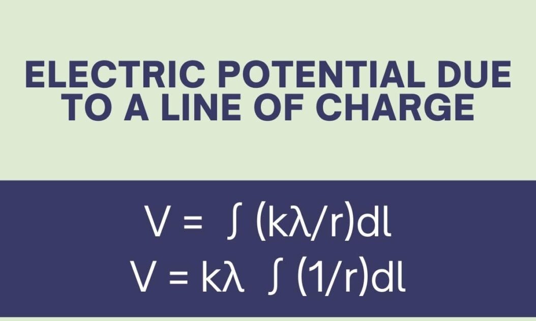
Electric Potential Due to Line Charge Equation
V = ∫(kλ/r)dl
V = kλ ∫(1/r)dl
Where:
- k = Coulomb’s constant (≈ 9 × 10⁹ N⋅m2/C2)
- λ = Linear charge density (C/m)
- r = Distance from charge element dl to reference point (m)
Let’s walk through an example scenario to help visualize this derivation.
Scenario: Calculating the Potential 10 m from a Line Charge
Suppose we want to find the electric potential due to a 2 m long line of charge with a linear charge density of 5 μC/m, located 10 m from our reference point P. What is the potential at point P?
Step 1: Identify the Variables
- λ = 5 μC/m
- L = 2 m
- r = 10 m (distance from P to line charge)
Step 2: Set Up the Integral
Plugging into our electric potential equation:
V = kλ ∫(1/r)dl
V = (9 × 10⁹ N⋅m2/C2 ) * (5 × 10⁻⁶ C/m) * ∫(1/10 m)dl
Step 3: Evaluate the Integral
Since the line charge has a constant linear density along its length, we can pull out the 1/r term. The remaining integral just sums to the total length L:
∫dl = L = 2 mWe’re left with:
V = (9 × 10⁹ N⋅m2/C2 ) * (5 × 10⁻⁶ C/m) * (1/10 m) * (2 m)
     = 9,000 V
So at point P, 10 m from a 2 m line charge, the electric potential is 9,000 V.
Understanding this straightforward line charge example provides a foundation for tackling more complex geometries. Now let’s dive deeper into some key details and considerations.
When Position Matters: Variations Based on Point Location
As we saw above, the electric potential depended heavily on the distance r from our reference point P to the line charge. If we changed the location of point P, the potential would also change. Let’s explore some of these location based variations.
Potential on the Perpendicular Bisector
If point P lies on the perpendicular bisector of the line charge, then the distance r is constant relative to all parts of the line. In this case, the integral simplifies to:
V = (kλL)/rOnly the total charge Q = λL and distance r matter. The length L cancels out.
Potential at the Endpoint of the Line
What if point P is located right at one end of the line charge? Now r varies depending on which charge element dl we consider. The full integral must be evaluated.
In this scenario, the potential becomes:
V = (kλ)ln(L/r)Where L/r represents the ratio of the full line length to the smallest distance r.
Potential Due to Multiple Line Charges
If multiple finite line charges are present, we simply sum the contributions from each one:
V = ∑(kλ<sub>i</sub>)ln(L<sub>i</sub>/r<sub>i</sub>) Where the index i refers to values for the ith line charge. This superposition of electric potential allows complex geometries to be broken down into simpler components.
Understanding how the potential equation changes for different point locations provides greater flexibility in solving problems. Next, let’s explore some interesting behaviors.
Strange Behaviors: Infinity and Beyond
Calculating electric potential can reveal some surprising behaviors not seen when working with the electric field alone. These typically arise for certain geometries when boundaries approach infinity. Some key examples include:
Infinite Line Charge
For an infinite line charge where L approaches infinity, the potential equation becomes:
V = (kλ)|z| Here z represents the perpendicular distance from the line charge. The absolute value accounts for position above or below the line along this z-axis.
We find that the potential increases linearly without bound, becoming infinite far from the line charge! This non physical prediction emphasizes that our equations eventually break down for extreme hypothetical cases.
Potential of a Ring
If we bend an infinite line charge into a ring or circle, our potential integral can still be solved. We find that the potential is zero anywhere inside the ring!
This strange consequence for continuous charge distributions contradicts our expectations about potentials arising from electric fields. Once again we encounter surprising non physical predictions from our mathematical equations under special geometries.
Dealing with these infinity issues leads into even more complex theoretical considerations that are beyond this introductory treatment. For now, these examples serve to expand our understanding of electric potential behavior in counterintuitive special cases involving lines or rings of charge.
Practical Applications: The Parallel Plate Capacitor
After exploring the conceptual basics with line charges, let’s turn our attention to one of the most common applications – the parallel plate capacitor. This system utilizes two large planar electrodes of opposite charge, essentially forming an approximation to finite parallel line charges. How do the potentials relate to real world capacitor behavior?
Capacitor Construction
A basic parallel plate capacitor consists of two metal plates with area A separated by small distance d. When connected to a battery, equal but opposite surface charge densities ±σ develop on each plate, resulting in uniform electric field lines between the plates.
Relation to Potential Difference
The oppositely charged plates produce an approximately uniform potential difference ΔV. By applying our line charge equations, it can be shown that the potential difference depends directly on the plate charge density and separation distance:
ΔV = σd/ε0Where ε0 represents the permittivity of space. For parallel plates, ΔV maps directly to voltage!
Capacitance and Charge Storage
This potential difference also allows us to introduce the concept of capacitance C:
C = Q/ΔV = ε0A/dWhere Q = total charge stored. This equation describes the charge storage ability of a capacitor through the geometric properties of its plates.
Analyzing parallel plate capacitors bridges the gap between conceptual line charge models and applications. The same principles of electric potential are key to understanding capacitor behavior.
History: Origins and Pioneers
The electric potential is closely tied to the history of concepts like voltage, energy, and capacitance. Let’s highlight some key contributors that advanced our understanding:
1700s – Alessandro Volta
Volta introduced the idea of an electrostatic “tension” to describe forces between charged objects, an early version of potential energy. His Voltaic piles led to the first electric batteries.
1785 – Charles Augustin de Coulomb
Coulomb devised experiments with a torsion balance to quantify the forces between point charges, leading to Coulomb’s law and the introduction of electric permittivity.
Early 1800s – Potential Coefficients
In the early 19th century, mathematical formulas were derived to calculate potentials by summing point charge contributions with respect to reference points. This established the coordinate potential theory we still use today.
1870s – James Clerk Maxwell
Maxwell incorporated electric and magnetic fields into a unified theory governed by differential equations. His work is the foundation of modern electrodynamics.
Conclusion
In summary, the electric potential forms a core concept linking electrostatic fields to energies, forces, voltage, and capacitance. While lines and rings of charge represent simplified models, the associated integrals and equations describe potentials in idealized scenarios. This establishes a mathematical foundation that can be extended to complex geometries. Studying the electric fields and potentials tied to these charge configurations provides crucial steps towards applied engineering with relevance.
So while the electric potential integral may seem abstract, it evolved naturally from centuries of experimental observations paired with mathematical physics. Today it remains an indispensable concept.
FAQs:
How are electric potential and electric field different?
While related, the electric potential represents energy per unit charge while the electric field reflects force per unit charge. Think of voltage versus current, different but complementary concepts.
Why does the potential equation depend on logs and integrals?
Integrals account for contributions from the continuous charge distribution along the line. Logs handle ratios and differences required to reference potentials to chosen points.
What happens inside a charged conductor?
The electric field is zero in electrostatic equilibrium, while the constant potential reflects the fixing of charges to the conducting surfaces.
Can electric potential be positive or negative?
Yes! The sign reflects whether charge is flowing to lower or higher potential regions relative to the reference point.
How do we calculate work or energy changes from potential?
Changes in potential ΔV between points directly give the change in electrical potential energy ΔU per unit charge: ΔU = qΔV.

- How to Enable Screen Sharing in Discord? – Guide - April 19, 2026
- How to Share Internet from Mobile to Mobile without Hotspot? - April 19, 2026
- 12 Best Janitor.Ai Alternatives (FREE) - April 18, 2026